


Introduction
Support Vector Machines (SVMs) represent a class of supervised learning models widely used for classification and regression tasks. Formulated within the framework of statistical learning theory, SVMs offer a robust approach to delineate decision boundaries by maximizing the margin between classes. At its core, SVMs aim to find the hyperplane that best separates data points into distinct classes while maximizing the margin, which is the distance between the hyperplane and the closest data points from each class, termed support vectors. This characteristic of SVM not only facilitates effective classification but also enhances generalization performance by minimizing overfitting.
In essence, SVMs encapsulate a mathematical representation of the solution space, making them particularly appealing for applications where data is not inherently linearly separable. Through the introduction of kernel functions, SVMs can be extended to handle non-linear relationships between the input features and target classes, thereby enhancing their versatility and applicability across diverse domains.
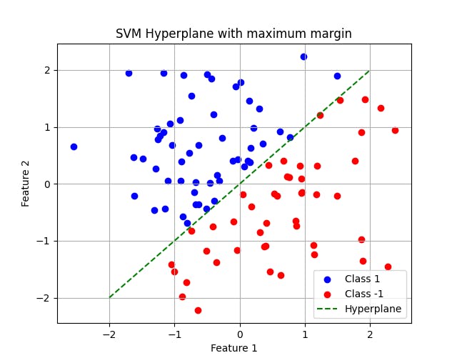
This visualization demonstrates the concept of margin maximization, where the hyperplane effectively separates the two classes while maximizing the margin between them. Such clear delineation is a hallmark of SVMs and underscores their utility in various machine learning tasks.
History
Support Vector Machines have roots dating back to the 1960s, emerging from the pioneering work of Vapnik and Chervonenkis in the Soviet Union. Initially proposed within the framework of statistical learning theory, SVMs gained traction due to their robust performance in classification tasks and theoretical underpinnings in optimization and statistical inferences.
The foundational concept of SVMs can be traced back to the perceptron, a precursor to modern neural networks, introduced by Frank Rosenblatt in 1957. While the perceptron laid the groundwork for binary classification, it was limited in its ability to handle nonlinear data distributions and prone to convergence issues.
The breakthrough for SVMs came in the 1990s when Vladimir Vapnik and Corinna Cortes introduced the optimal hyperplane algorithm for binary classification. This algorithm sought to find the hyperplane that maximized the margin between classes, thereby enhancing generalization performance and mitigating overfitting. The formulation of SVMs as a convex optimization problem paved the way for efficient training algorithms and widespread adoption in various domains including image recognition, bioinformatics, and financial forecasting.
Over the years, SVMs have undergone significant advancements, including the introduction of kernel methods by Bernhard Boser, Isabelle Guyon, and Vladimir Vapnik in 1992. Kernel methods allowed SVMs to operate in high-dimensional feature spaces and accommodate nonlinear relationships between input features and target classes. This extension further solidified the position of SVMs as a versatile tool in the machine learning toolkit.
The evolution of SVMs continues to this day, with ongoing research focusing on scalability, interpretability, and adaptation to emergin data modalities. Despite the emrgence of newer algorithms and techniques, SVMs remain a cornerstone of modern machine learning.
Mathematical Foundation of SVM
Support Vector Machines (SVMs) are grounded in the principles of statistical learning theory, aiming to discern decision boundaries between classes while maximizing the margin between them. Central to SVMs is the notion of hyperplanes and margin maximization.
Hyperplanes:
In SVMs, a hyperplane is a flat affine subspace of dimension one less than than the feature vector space. For a dataset with \(n\) features, the hyperplane is represented as \(n-1\) dimensional subspace. In a binary classification scenario, a hyperplane serves as the decision boundary that separates data points belonging to different classes. Mathematically, a hyperplane in \(n\)-dimensional vector space is defined by the equation:
$$w^T \cdot x + b = 0$$
where \(w\) is the weight vector perpendicular to the hyperplane, \(x\) is the input feature vector, and \(b\) is the bias term.
Margin Maximization:
The key objective of SVMs is to identify the hyperplane that maximizes the margin between the classes. The margin is the distance between the hyperplane and the closest data points from each class, termed support vectors. Maximizing the margin ensures generalization performance and resilience to noise.
Support Vectors:
Support vectors are the data points closest to the decision boundary (hyperplane) and have non-zero weights in the SVM model. These points play a crucial role in defining margin and determining the optimal hyperplane.
Formulation of the Optimization Problem:
In its simplest form, the optimization problem of SVMs involves finding the hyperplane that separates the data with the maximum margin. Mathematically, this can be formulated as a constrained optimization problem:
$$\text{Minimize } \frac{1}{2}||w||^2$$
subject to:
$$y_i (w^T \cdot x_i + b) \ge 1 \text{ for all i=1,2,..,n}$$
where \(||w||\) denotes the Euclidean norm of the weight vector, \(x_i\) represents the \(i^{th}\) input feature vector, and \(y_i\) denotes the corresponding class label \((y_i \in \{-1, 1\})\).
Soft Margin SVM:
In real-world scenarios, data may not be perfectly separable. To handle such cases, a soft margin SVM introduces a slack variable \((\xi_i) \) for each data point, allowing for misclassifications. The optimization is modified as follows:
$$\text{minimize } \frac{1}{2} ||w||^2 + C \sum_{i=1}^{n}\xi_i$$
subject to:
$$y_i(w^T \cdot x_i + b) \ge 1 - \xi_i \text{ and } \xi_i \ge 0 \text{ for all i=1,...,n}$$
where \(C\) is the regularization parameter that controls the tradeoff between maximizing the margin and minimizing the classification error.
Kernel Tricks and Nonlinear SVMs
While traditional SVMs are effective for linearly separable data, many real-world datasets exhibit nonlinear relationships between input features and target classes. To address this limitation, SVMs leverage kernel tricks, enabling them to operate in higher-dimensional feature spaces and capture complex decision boundaries.
Introduction to Kernel Methods:
Kernel methods are a fundamental component of nonlinear SVMs, allowing for the implicit mapping of input features into a higher-dimensional space where the data may be linearly separable. The key idea behind kernel methods is to compute the dot product between feature vectors in this higher-dimensional space without explicitly performing the transformation. This approach circumvents the computational load associated with explicitly transforming the data into higher dimensions.
Kernel Functions:
A kernel function \((K)\) computes the dot product between the feature vectors in the higher-dimensional space. Commonly used kernel functions include:
Linear Kernel: \(K(x, x') = x^T \cdot x'\)
Polynomial Kernel: \(K(x, x') = (x^T \cdot x' + c)^d\)
Radial Basis Function (RBF) Kernel: \(K(x, x') = e^{-\gamma||x-x'||^2}\)
where \(x\) and \(x'\) are input feature vectors, \(c\) is a constant, \(d\) is the degree of the polynomial, and \(\gamma\) is a parameter controlling the smoothness of the decision boundary.
Implicit Mapping:
The key insight of kernel methods is that dot product in the higher-dimensional space that can be computed efficiently without explicitly transforming the data. This is achieved by defining a kernel function that captures the desired similarity measure between feature vectors. By computing the dot product implicitly through the kernel function, SVMs can operate in the higher-dimensional space without incurring the computational cost of explicitly transforming the data.
Example:
Suppose our dataset is given as \(\{(-5, -1), (-4, -1), (-3, -1), (-2, 1), (-1, 1), (0, 1), (1, 1), (2, 1), (3, -1), (5, -1) \}\)
This dataset can be projected in a one-dimensional vector space as:
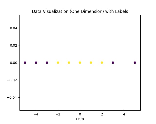
As you can see, there is no line that can separate the yellow and violet dots in the one-dimensional feature space. One kernel trick is to add a second dimension with the transformation \(f(x) = x^2\) and then try to visualize the data in this two-dimensional feature space as:
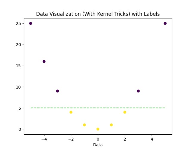
As you can see, the green-dotted line can now separate the data points in this higher-dimensional space very easily. This is the advantage of Kernel tricks where data points when projected to a higher-dimensional space make the data linear in nature.
Optimization and Training
The optimization and training of SVMs involve solving a constrained optimization problem to find the optimal hyperplane that maximally separates the classes while minimizing the classification errors. This section will delve into the mathematical formulation of the optimization problem and explore various techniques for solving it efficiently.
Formulation of the Optimization Problem:
Mathematically, the primal form of the optimization problem is formulated as:
$$\text{minimize } \frac{1}{2} ||w|| ^ 2$$
subject to the constraints:
$$y_i(w^T \cdot x_i + b) \ge 1 \text{ for all i=1,...,n}$$
Lagrange Duality:
To navigate through the constrained optimization efficiently, SVMs use Lagrange duality. By introducing Lagrange multipliers \((\alpha_i)\) for the inequality constraints, the problem is transformed into its dual form. This involves constructing a Lagrangian function:
$$L(w, b, \alpha) = \frac{1}{2}||w||^2 - \sum_{i=1}^{n} \alpha_i(y_i(w^T \cdot x_i + b) - 1)$$
Derivation of the Dual Problem:
The maximization of the Lagrangian with respect to \(\alpha\) subject to Karush-Kuhn-Tucker (KKT) conditions leads to the formula of the dual problem:
$$\text{maximize } \Theta(\alpha) = \sum_{i=1}^n \alpha_i - \frac{1}{2} \sum_{i=1}^n \sum_{j=1}^n \alpha_i \alpha_j y_i y_j x_i^Tx_j$$
subject to:
$$\alpha_i \ge 0 \text{ for all i=1,...,n}$$
$$ \sum_{i=1}^n \alpha_i y_i = 0$$
Solution of the Dual Problem:
Various optimization techniques such as Sequential Minimal Optimization (SMO) or Quadratic Programming (QP) are employed to solve the dual problem efficiently. Upon obtaining the optimal values of \(\alpha\), the weight vector \(w\) and bias term \(b\) are derived.
Kernel Trick and Mercer's Theorem:
To accommodate nonlinear data, SVMs leverage kernel functions, avoiding the explicit transformation of features into higher dimensions. Mercer's theorem ensures that any positive semi-definite kernel function corresponds to a valid inner product in some vector space, allowing for the utilization of the kernel trick seamlessly.
Training
The training process of SVMs involves several steps aimed at finding the optimal hyperplane. The training algorithm is as follows:
Preprocess the training data: Before training the SVM model, it is essential to preprocess the training data. This may involve steps such as normalization, scaling, or handling missing values to ensure that the input features are in a suitable format for training. Preprocessing helps in improving the convergence of the optimization algorithm and enhances the overall performance of the SVM model.
Formulating the Optimization Problem: The core of SVM training lies in formulating the optimization problem, typically in its dual form. The primal form seeks to minimize the norm of the weight vector subject to constraints, while the dual form maximizes a function of Lagrange multipliers subject to certain conditions. The choice between the primal and dual forms depends on factors such as computational efficiency and the specific problem at hand.
Solving the Dual Problem: Once the optimization problem is formulated, it needs to be solved to obtain the optimal values of the Lagrange multipliers \(\alpha\). Various optimization techniques can be employed for this purpose, such as Sequential Minimal Optimization (SMO) or Quadratic Programming (QP). These techniques iteratively update the Lagrange multipliers to converge to their optimal values, thereby determining the support vectors and the parameters of the decision boundary.
Computing the Weight Vector and Bias Term: With the optimal values of \(\alpha\)obtained, the weight vector \(w\) and bias term \(b\) of the hyperplane can be computed. The weight vector \(w\) is a linear combination of the support vectors weighted by their corresponding Lagrange multipliers \(\alpha\). The bias term \(b\) is computed using the Karush-Kuhn-Tucker (KKT) conditions to satisfy the margin constraints.
Classification of New Data Points: Once the SVM model is trained and the parameters (\(w\) and \(b\)) are determined, it can be used to classify new data points. Given a new data point \(x\), its class label is predicted by evaluating the sign of the decision function:
$$f(x) = sign(w^T \cdot x + b)$$
- Evaluation and Fine Tuning: After training and classification, it's essential to evaluate the performance of the SVM model using appropriate metrics such as accuracy, precision, recall, or F1-score. Depending on the performance, the model may be fine-tuned by adjusting hyperparameters such as the regularization parameter (C) or the choice of kernel function. This iterative process helps in optimizing the SVM model for better generalization performance on unseen data.
Conclusion
In conclusion, Support Vector Machines (SVMs) represent a powerful class of supervised learning models that excel in classification tasks by effectively delineating decision boundaries between classes. Stemming from the foundations of statistical learning theory, SVMs offer a robust framework for binary and multiclass classification, with the ability to handle both linearly separable and nonlinear data distributions.
Throughout this article, we have explored the mathematical underpinnings of SVMs, including the concepts of hyperplanes, margin maximization, Lagrange duality, and kernel tricks. We have elucidated the optimization and training algorithm, detailing the steps involved in formulating the optimization problem, solving it using optimization techniques, and computing the parameters of the decision boundary.
Furthermore, we have discussed the versatility of SVMs in handling nonlinear data through kernel methods, which allow for the implicit mapping of input features into higher-dimensional spaces. The kernel trick enables SVMs to capture complex decision boundaries without explicitly transforming the data, thereby enhancing their applicability across diverse datasets and domains.
Despite the emergence of newer machine learning algorithms, SVMs remain a cornerstone of modern machine learning, owing to their solid theoretical foundation, robust performance, and interpretability. As researchers continue to explore advancements in optimization techniques, kernel methods, and scalability, SVMs are poised to remain relevant in the ever-evolving landscape of machine learning.
In essence, understanding Support Vector Machines from a mathematical perspective offers insights into their inner workings and empowers practitioners to leverage their capabilities effectively. Whether in academia, industry, or research, SVMs continue to be indispensable tools for tackling classification challenges and advancing the frontiers of machine learning. As we embark on this journey of exploration and innovation, let us continue to harness the power of SVMs to unlock new possibilities and drive progress in artificial intelligence and beyond.